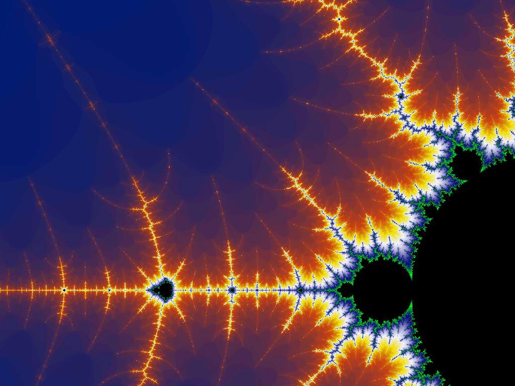
Hyperbolic numbers and fractals

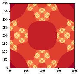
What happens when we change the identity defining the imaginary unit for the complex numbers $i^2=-1$ to $i^2=1$ and enforcing i different from 1? We get the somewhat less known numbers called hyperbolic or split-complex numbers. The most common thing about complex numbers that comes to mind are the nice pictures of fractals and there are plenty of tools already out there to generate them. However, for the hyperbolic numbers there aren't as much fractal generators out there, so let us now make a simple tool in Python to generate these fractals as well.

First, we need to implement the basic arithmetic with hyperbolic numbers. This will enable us to write simple arithmetic expressions like z**2 + c directly instead of writing out the expressions in component form using real and imaginary parts. I made a simple Python implementation of class HyperbolicNumber in module hyperbolic doing exactly this. Using this module, we can now write a function for counting the number of iterations of f(z)=z**2+c before "escaping to infinity" in a straightforward way. In fact the formula is identical to the escape-time algorithm for fractals over complex numbers.

from hyperbolic import HyperbolicNumber

def f(z):
    w = z
    total = 0
    while mag(w) < 2.0 and total < 300:
        w = w**2 + z
        total += 1
    return total

Basically, the above function is all we need to start generating images of fractals. Here of course, we focus only on the famous map family { f_c(z) = z**2+c} indexed by c, but any other could be used as well. We add an additional parameter to f(z) to become f(z,c) and encapsulate it in the HyperbolicFractal class. This class will be our abstraction for a fractal calculation, which basically just calculates a 2**-k approximation of the Julia set of f_c over some given rectangular region in the hyperbolic number plane. For all the points z of a given rectangular range [centerx-rangex, centerx+rangex]x[centery-rangey, centery+rangey] we perform the call to f(z, c). To avoid recalculation every time of the same region, or part of a region, points which have already been calculated are stored in an internal cache so any subsequent calls to f(z, c) are just looked up instead of being recalculated. Here's the code.

import numpy
import matplotlib.cm as cm
import matplotlib.pylab as plt
from hyperbolic import HyperbolicNumber

class HyperbolicFractal:
    def __init__(self):
        self.hits = 0
        self.cache = {}
        
    def f(self, z, c):
        if (z, c) in self.cache:
            self.hits += 1
            return self.cache[(z, c)]
        w = z
        total = 0
        while mag(w) < 2.0 and total < 300:
            w = w**2 + c
            total += 1
        self.cache[(z, c)] = total
        return self.cache[(z, c)]

    def show(self, scale, centerx, centery, rangex, rangey, c):
        """Draw a 2**(-scale) approximation of a hyperbolic fractal 
        over a given rectangular range."""
        self.hits = 0
        totals = (centerx+rangex - (centerx-rangex))\
        * (centery+rangey - (centery-rangey))
        t = [[self.f((1.0/(2**scale)) * HyperbolicNumber(x,y), c)\
        for x in range(centerx-rangex, centerx+rangex)]\
        for y in range(centery-rangey, centery+rangey)]
        matrix = numpy.matrix(t)
        fig = plt.figure()
        plt.imshow(matrix, interpolation='bilinear', cmap=cm.RdYlGn, origin='center')
        print ("Total: {} Cache hits: {} Cache hit ratio: {}".format(totals, self.hits, (1.0 * self.hits)/totals))
        plt.show()

Let's try it out.

H = HyperbolicFractal()
H.show(7, 0, 0, 200, 200, HyperbolicNumber(-20/2**3, 0))

And there you have it! We now have a tool to look into the hyperbolic number world.

The full code for this implementation can be found on Github.

Computable Sets in the Euclidean plane using Python

#####################################################################
#
# Implementing the notion of Computable Set in the euclidean plane 
#
# Every weakly computable set in the euclidean plane is a set 
# of zeroes of some a computable function.
#
# Konrad Burnik, June 2017.
#
#####################################################################

from math import *
from decimal import *
import matplotlib.pyplot as plt

class ComputableSet:
    '''A computable subset of the euclidean plane is given by its computable function representing it.'''
    def f(self, x, y):
        '''A function whose zeroes represent this computable set. 
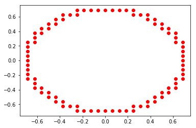
           For example: def f(x, y): return x**2 + y**2 - 1 has zeroes which represents a unit circle.
        '''
        raise Exception("Not implemented!")
    
    def points(self, k):
        return [(x/2**k, y/2**k) 
                        for y in range(-2**k, 2**k + 1) 
                        for x in range(-2**k, 2**k + 1) 
                        if Decimal(-1) / Decimal(2**k) < self.f(Decimal(x)/Decimal(2**k), Decimal(y)/Decimal(2**k)) < Decimal(1) / Decimal(2**k)]  class Circle(ComputableSet):
    def f(self, x, y):
        return x**2 + y**2 - Decimal(1/2)
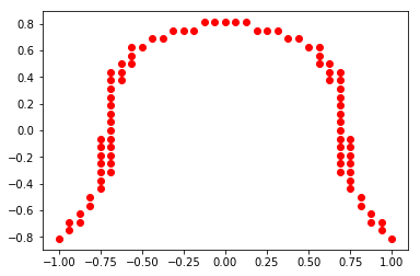
class EllipticCurve(ComputableSet):
    def f(self, x, y):
        return x**2 + y**3 - Decimal(1/2)

def plot_set(s, k):
    points = s.points(k)
    x = list(map(lambda x : x[0], points))
    y = list(map(lambda x : x[1], points))

    plt.plot(x, y, 'ro')
    plt.show()

class Circle(ComputableSet):
    def f(self, x, y):
        return x**2 + y**2 - Decimal(1/2)

class EllipticCurve(ComputableSet):
    def f(self, x, y):
        return x**2 + y**3 - Decimal(1/2)

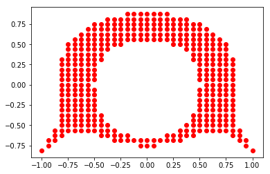
class ComputableSetUnion(ComputableSet):
    def __init__(self):
        self.A = ComputableSet()
        self.B = ComputableSet()
        
    def f(self, x, y):
        return self.A.f(x, y) * self.B.f(x, y)

Computable metric spaces in a nutshell

Leave a reply

What are computable metric spaces?

We can generalize the notions of computability over the reals and in the euclidean space to metric spaces. A computable metric space is a triple $(X,d,\alpha)$ where $(X,d)$ is a metric space and $\alpha$ is a sequence in $X$ such that its image is dense in $X$ and the function $\mathbb{N}^2 \rightarrow \mathbb{R}$ defined as $(i,j) \mapsto d(\alpha_i, \alpha_j),\ \forall i,j\in\mathbb{N}$ is computable. For example, a definition of computable point is a generalization of the computable real: A point $x \in X$ is computable in $(X,d,\alpha)$ if there exists a computable function $f:\mathbb{N} \rightarrow \mathbb{N}$ such that $d(\alpha_{f(k)}, x) < 2^{-k}$ for every $k \in \mathbb{N}$ . Similarly, we can define a computable sequence of points in $X$ and functions between metric spaces that are computable,... but for subsets of $X$ it is not the same as definition of computability in $\mathbb{R}^n$ but it borrows the definitions from classical recursion theory. First we fix some computable enumeration of rational balls in $X$ for example let $(I_i)$ be a fixed such enumeration. Then for a set $S \subseteq X$ we say that $S$ is recursively enumerable $T = \{i \in \mathbb{N} | S \cap I_i \not = \emptyset\}$ is recursively enumerable i.e. there exists a computable function $f:\mathbb{N} \rightarrow \mathbb{N}$ such that $f(\mathbb{N}) = T$ . A subset $S$ is co-recursively enumerable if we have an algorithm that covers the complement of $S$ with rational balls. In other words, $S$ is co-recursively computable iff there exists a recursively enumerable subset $A$ of $\mathbb{N}$ such that $X \setminus S = \bigcup_{i \in A} I_i$ . A subset $S$ is computable iff $S$ is recursively computable and co-recursively computable.

We can of course generalize further and define computable topological spaces but I shall not go further into that. That is a topic for another post. Note that as we generalize more and more there are pathological spaces that do not have nice computability properties and must be more and more careful when dealing with computability.

Introduction to computable analysis (Part 1/2)

Leave a reply

What is Computable analysis anyway?

Roger Penrose in his book "The emperors new Mind" asked an interesting question regarding the Mandelbrot set: "Is the Mandelbrot set recursive?" The term "recursive" is an old name for "computable" and has nothing to do with recursion in programming.

The Mandelbrot Set (zoomed in)

Classical computability theory (also known as recursion theory) is a branch of mathematical logic that deals with studying what functions $\mathbb{N}\rightarrow \mathbb{N}$ are computable. Computable analysis is in some sense an extension of this theory. It is a branch of mathematics that applies computability theory to problems in mathematical analysis. It is concerned with questions of effectivity in analysis and its main goal is to find what parts of analysis can be described by an algorithmic procedure, one of the basic questions being what functions $f:\mathbb{R}\rightarrow\mathbb{R}$ are computable? (note the domain and codomain are now the reals).

Computable reals

Suppose we take a real number $x$ . Is $x$ computable? What do we mean by $x$ being computable? If we can find an algorithm $A$ that calculates for each input $k \in \mathbb{N}$ a rational approximation $A_k$ of $x$ ; and such that the sequence $(A_k)$ "converges fast" to $x$ then we say that $x$ is a computable real. More precisely, a real number $x \in R$ is computable iff there exists a computable function $f:\mathbb{N} \rightarrow \mathbb{Q}$ such that $|f(k) - x| < 2^{-k}$ for each $k \in \mathbb{N}$ . For example, every rational number is computable. The famous number $\pi$ is computable, and in our previous post we proved that $\sqrt{2}$ is computable. It turns out that the set of computable reals, denoted by $\mathbb{R}_C$ is a field with respect to addition and multiplication. But there exist real numbers which are not computable. This is easy to see as there is only a countable number of computable functions $\mathbb{N}\rightarrow\mathbb{N}$ , and since we know that $\mathbb{R}$ is uncountable, so we have more real numbers than we have possible algorithms, we conclude that there must be a real number that is not computable. One example of an uncomputable real is the limit of a Specker sequence. And one other interesting one is the Chaitin constant. In fact, if we take any recursively enumerable but non-recursive set $A \subseteq \mathbb{N}$ , then the number $\alpha = \sum_{i \in A} 2^{-i}$ is an example of a real number which is not computable.

Computable sequences of reals

If we have a sequence of computable reals $(x_n)$ (and hence a sequence of algorithms) we may ask if this sequence is computable i.e. is there a single algorithm that describes the whole sequence? If there exists a computable function $f : \mathbb{N}^2 \rightarrow \mathbb{Q}$ such that

$|f(n,k) - x_n| < 2^{-k}$

for each $n,k \in \mathbb{N}$ then we say that $(x_n)$ is a computable sequence of reals. We have seen that each rational number is computable, but this is not true for sequences of rational numbers! One example of a sequence that has each term computable and also computable as a sequence of reals, but it is not computable as a sequence of rationals is the following [Pour-el, Richards]:

Example:

Take any recursively enumerable but non-recursive set $A \subseteq \mathbb{N}$ and let $a:\mathbb{N} \longrightarrow \mathbb{N}$ be a one-to-one recursive function which enumerates $A$ .

Let $f:\mathbb{N} \longrightarrow \mathbb{Q}$ be given by

$f(n) = 2^{-m}, \mbox{ if } m = a(n) \mbox{ for some } m \\, 0 \mbox{ otherwise. }$

Then $f$ is not computable (as a sequence) of reals but $f$ is not computable as a sequence of rationals.

Computable real functions

Real functions which are the main object of study in analysis can be studied in this computability setting, a function $f:\mathbb{R} \rightarrow \mathbb{R}$ is computable iff

it maps computable sequences to computable sequences i.e. $f(x_i)$ is computable for every computable sequence $(x_i)$ ;
it is effectively uniformly continuous;

The fundamental theorem of computable analysis is that every computable real function is continuous.

There is also a notion of computability for the process of integration, derivation, solving partial differential equations, etc. and we shall look into that topic in another post.

Computable subsets of the Euclidean space

Unit circle approximated with dyadic points

Next, let's look at the subsets of the euclidean space $\mathbb{R}^n$ and ask a simple question: what subsets are computable? First, note that saying $S$ is computable iff its indicator function

$\chi_S(x) =\begin{cases} 1, & x \in S \\ 0, & x \not \in S \end{cases}$

is computable is not a useful definition since the indicator function is not continous except when $S =\mathbb{R}^n$ or $S=\emptyset$ . A subset $S$ of $\mathbb{R}^n$ is computable iff the function $\mathbb{R}^n \rightarrow \mathbb{R}$ defined as $x \mapsto d(x, S)$ is a computable function. For example, take the unit circle in $\mathbb{R}^2$ .

$\mathbb{S}^1 = \{(x,y): x^2 + y^2 =1\}$

. The distance function is

$d((x,y), \mathbb{S}^1) = |x^2 + y^2 - 1|, \forall x,y \in \mathbb{R}^2.$

These are just some basic definitions and facts, but also interesting questions are studied in computable analysis like for example what mappings preserve computability of objects? Is for example the Mandelbrot set computable? What about Julia Sets? For them, there are nice results presented in the book "Computability of Julia Sets" by Braverman and Yampolsky. Although Julia Sets have been thoroughly researched in the book, for the Mandelbrot set we still don't know the answer.

Basically for anything we do in analysis (finding derivatives, integration, finding roots, solving PDEs ...) we may ask: "Is it computable?" and that is a topic for another post.

(to be continued)

Another look at the square root of two

Leave a reply

The other day I was thinking about approximating $\sqrt{2}$ in terms of segments of size $1/2^k$ for $k=0,1,2,\dots$ , The question I was interested was "What is the least number of segments of length $1/2^k$ that we need to cross over $\sqrt{2}$ starting from zero?" and one particular sequence of integers I came up with was this:

$2, 3, 6, 12, 23, 46, 91, 182, 363, 725,\dots.$

Sadly, at the time of writing this post the Online Encyclopedia of Integer Sequences did not return anything for this sequence.

The sequence represents the numerators for dyadic rationals which approximate $\sqrt{2}$ within precision $2^{-k}$ (within k-bits of precision), but is this sequence computable? In what follows I assume that the reader is familiar with the basic definitions of mu-recursive functions.

It turns out that our sequence can be described by a recursive function $f: \mathbb{N} \rightarrow \mathbb{N}$

$f(k) = \mu.n [n^2 > 2^{(2k+1)}]$

for all $k\geq0$ .

The idea of the function $f$ is that for each $k$ it outputs the number of $1/2^k$ segments that fit into $\sqrt{2}$ plus one.

Since for each $k$ , the value $f(k)$ is the smallest integer such that $f(k)/2^k > \sqrt{2}$ we have

$(f(k) - 1)/2^k < \sqrt{2} < f(k)/2^k$

for each $k\geq 0$ .

From this we obtain the error bound $|f(k)/2^k - \sqrt{2}| < 2^{-k}$ .

Approximation of $\sqrt{2}$ within precision $2^{-k}$ can be "represented" by a natural number $f(k)$ . To get the actual approximation by a dyadic rational just divide by $2^k$ but what we want is to avoid division. We want to calculate only with natural numbers!

Implementation

The function f has a straightforward (although inefficient) implementation in Python.

def calcSqrt2Segments(k):
    n = 0
    while(n*n <= 2**(2*k+1)):
        n = n + 1
    return n

This is in fact terribly inefficient, but in computability theory efficiency is not the goal, the goal is usually to prove that something is uncomputable even if you have all the resources of time and space at your disposal. Nevertheless, here is a slightly better version we get if we notice that the next term $f(k+1)$ is about twice as large as $f(k)$ with a small correction.

def calcSqrt2segmentsRec(k):
    if k == 0:
        return 2
    else:
        res = 2*calcSqrt2segmentsRec(k-1) - 1
        if res*res <= 2**(2*k+1):
           res = res + 1
        return res

This of course suffers from stack overflow problems, so memoization is a natural remedy.

def calcSqrt2segmentsMemo(k):
    m = dict()
    m[0] = 2
    for j in range(1, k+1):
        m[j] = 2*m[j-1] - 1
        if m[j]*m[j] <= 2**(2*j+1):
            m[j] = m[j] + 1
    return m[k]

Memoization can use-up memory and we can do better. We don't need to memorize the whole sequence up to k to calculate $f(k+1)$ we only need the value $f(k)$ .

def calcSqrt2segmentsBest(k):
    m = 2
    for j in range(1, k+1):
        m = 2*m - 1
        if m*m <= 2**(2*j+1):
            m = m + 1
    return m

After defining a simple timing function and testing our memoization and "best" version we see that the best version is not so good in terms of running time when compared with memoization, they are both approximately about the same in terms of speed (the times are in seconds):

>>> timing(calcSqrt2segmentsMemo, 10000)
0.6640379428863525
>>> timing(calcSqrt2segmentsBest, 10000)
0.6430368423461914
>>> timing(calcSqrt2segmentsMemo, 20000)
3.3311898708343506
>>> timing(calcSqrt2segmentsBest, 20000)
3.3061890602111816
>>> timing(calcSqrt2segmentsMemo, 30000)
8.899508953094482
>>> timing(calcSqrt2segmentsBest, 30000)
8.848505973815918
>>> timing(calcSqrt2segmentsMemo, 50000)
30.04171895980835
>>> timing(calcSqrt2segmentsBest, 50000)
29.96371293067932
>>> timing(calcSqrt2segmentsMemo, 100000)
164.99343705177307
>>> timing(calcSqrt2segmentsBest, 100000)
168.6026430130005

Neverteless, we can use our "best" program to calculate $\sqrt{2}$ to arbritrary number of decimal places (in base 10). First, we need to determine how many bits are sufficient to calculate $\sqrt{2}$ to $n$ decimal places in base 10. Simple calculation yields:

$k > \lceil n log_2 10 \rceil.$

In Python we need a helper function that calculates this bound that avoids the nasty log and ceiling functions, so here it is:

def calcNumDigits(n):
    res = 1
    for j in range(2, n+1): 
        if( j%3 == 0 or j%3 == 1 ):
          res = res + 3
        else:
          res = res + 4
    return res

At last, calculating $\sqrt{2}$ to arbritrary precision is done with this simple code below, returning a String with the digits of $\sqrt{2}$ in base 10. Note once more, that all this calculation is done only with the natural numbers and here we are using Python's powerful implementation of arithmetic with arbritrary long integers (which is not as nicely supported for decimals at least at the time of writing this post).

Note also, that instead of dividing $f(k)$ by $2^k$ we are multiplying it with $5^k$ to get a natural number with all of it's digits being an approximation of $\sqrt{2}$ with k bits of precision. This natural number we are then converting to a string, inserting a decimal point '.' and returning this as our result. So, here is the code:

def calcSqrt2(n):
    k = calcNumDigits(n)
    res = str(5**k * calcSqrt2segmentsBest(k))
    return res[0:1] + '.' + res[1:n]

Running it gives us nice results:

>>> calcSqrt2(30)
'1.41421356237309504880168872421'
>>> calcSqrt2(300)
'1.41421356237309504880168872420969807856967187537694807317667973799073247846210703885038753432764157273501384623091229702492483605585073721264412149709993583141322266592750559275579995050115278206057147010955997160597027453459686201472851741864088919860955232923048430871432145083976260362799525140799'
>>> calcSqrt2(3000)
'1.41421356237309504880168872420969807856967187537694807317667973799073247846210703885038753432764157273501384623091229702492483605585073721264412149709993583141322266592750559275579995050115278206057147010955997160597027453459686201472851741864088919860955232923048430871432145083976260362799525140798968725339654633180882964062061525835239505474575028775996172983557522033753185701135437460340849884716038689997069900481503054402779031645424782306849293691862158057846311159666871301301561856898723723528850926486124949771542183342042856860601468247207714358548741556570696776537202264854470158588016207584749226572260020855844665214583988939443709265918003113882464681570826301005948587040031864803421948972782906410450726368813137398552561173220402450912277002269411275736272804957381089675040183698683684507257993647290607629969413804756548237289971803268024744206292691248590521810044598421505911202494413417285314781058036033710773091828693147101711116839165817268894197587165821521282295184884720896946338628915628827659526351405422676532396946175112916024087155101351504553812875600526314680171274026539694702403005174953188629256313851881634780015693691768818523786840522878376293892143006558695686859645951555016447245098368960368873231143894155766510408839142923381132060524336294853170499157717562285497414389991880217624309652065642118273167262575395947172559346372386322614827426222086711558395999265211762526989175409881593486400834570851814722318142040704265090565323333984364578657967965192672923998753666172159825788602633636178274959942194037777536814262177387991945513972312740668983299898953867288228563786977496625199665835257761989393228453447356947949629521688914854925389047558288345260965240965428893945386466257449275563819644103169798330618520193793849400571563337205480685405758679996701213722394758214263065851322174088323829472876173936474678374319600015921888073478576172522118674904249773669292073110963697216089337086611567345853348332952546758516447107578486024636008344491148185876555542864551233142199263113325179706084365597043528564100879185007603610091594656706768836055717400767569050961367194013249356052401859991050621081635977264313806054670102935699710424251057817495310572559349844511269227803449135066375687477602831628296055324224269575345290288387684464291732827708883180870253398523381227499908123718925407264753678503048215918018861671089728692292011975998807038185433325364602110822992792930728717807998880991767417741089830608003263118164279882311715436386966170299993416161487868601804550555398691311518601038637532500455818604480407502411951843056745336836136745973744239885532851793089603738989151731958741344288178421250219169518755934443873961893145499999061075870490902608835176362247497578588583680374579311573398020999866221869499225959132764236194105921003280261498745665996888740679561673918595728886424734635858868644968223860069833526427990562831656139139425576490620651860216472630333629750756978706066068564981600927187092921531323682'

Note:
This can of course be generalized to calculating the square root of any number and of any order. This is an easy exercise for the reader.

Computable Analysis Applied to Formal Verification of Cyber-Physical Systems

Leave a reply

The following video I found online is about combining the theory of computable analysis with formal verification methods. I find this video very interesting because my diploma/master's thesis was about formal verification while my PhD study is from the area of computable analysis, so the work presented in this video nicely combines the two areas.

Title: "Computable Real Numbers and Why They Are Still Important Today"

Author: Edmund Clarke

Description: "Talk by ACM A.M. Turing Laureate Edmund Clarke during the ACM A.M. Turing Centenary Celebration, June, 2012. Abstract: Although every undergraduate in computer science learns about Turing Machines, it is not well known that they were originally proposed as a means of characterizing computable real numbers. For a long time, formal verification paid little attention to computational applications that involve the manipulation of continuous quantities, even though such applications are ubiquitous. In recent years, however, there has been great interest in safety-critical hybrid systems involving both discrete and continuous behaviors, including autonomous automotive and aerospace applications, medical devices of various sorts, control programs for electric power plants, and so on. As a result, the formal analysis of numerical computation can no longer be ignored. This talk focuses on one of the most successful verification techniques, temporal logic model checking. Current industrial model checkers do not scale to handle realistic hybrid systems. The key to handling more complex systems is to make better use of the theory of the computable reals, and computable analysis more generally. New formal methods for hybrid systems should combine existing discrete methods in model checking with new algorithms based on computable analysis. In particular, this talk discusses a model checker currently being developed along these lines."

Links

CCA 2013 Conference

Leave a reply

I attended the Tenth International Conference on Computability and Complexity in Analysis in Nancy, France, with my PhD advisor Zvonko Iljazović, where I presented our joint work about the computability aspects of topological rays and lines in computable metric spaces. The link to the presentation slides can be found here.

CCA_2013_Topological_rays_and_lines_as_c

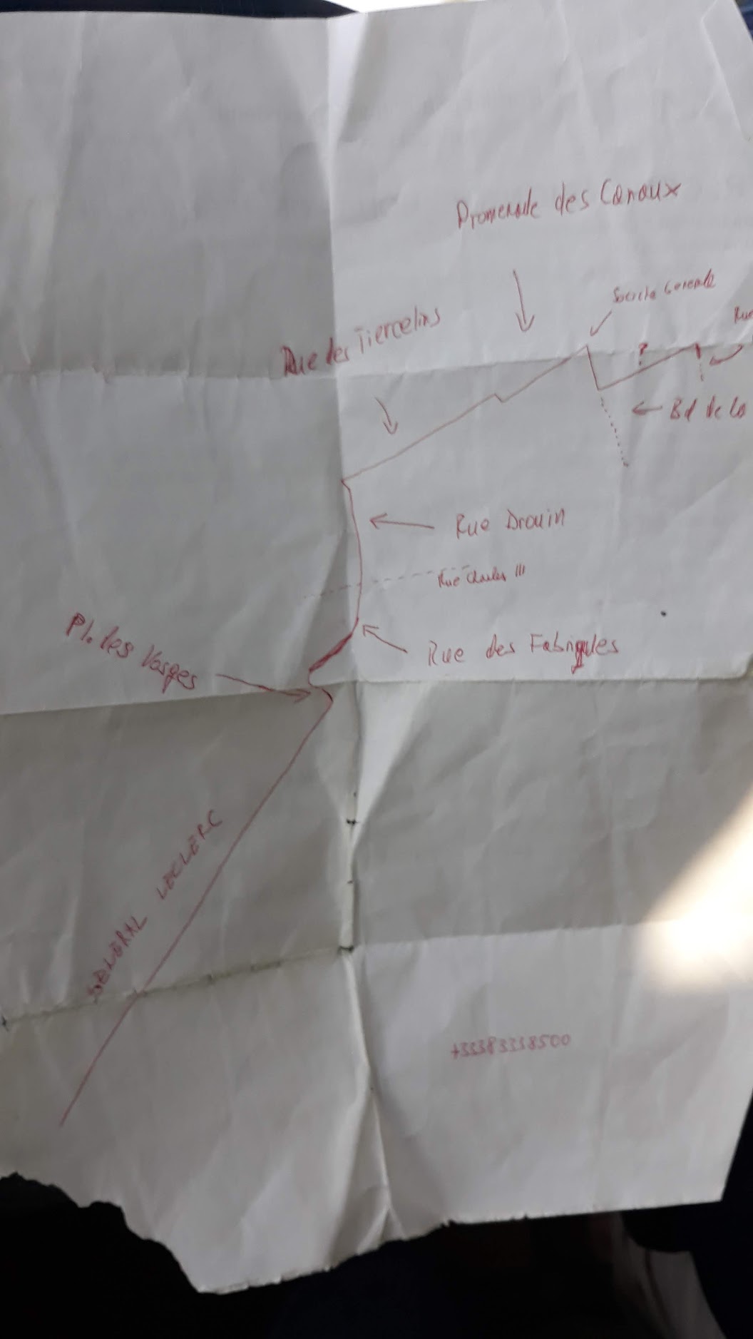
Below is a hand-drawn map that explains how to get from the hotel to the conference venue, hand-drawn by Zvonko. I kept it as a souvenir.