The other day I was thinking about approximating  in terms of segments of size
  for
for  , The question I was interested was "What is the least number of segments of length that we need to cross over starting from zero?" and one particular sequence of integers I came up with was this:
![\[2, 3, 6, 12, 23, 46, 91, 182, 363, 725,\dots.\]](https://konrad.burnik.org/wordpress/wp-content/ql-cache/quicklatex.com-e0fc94c01da00342e00775693d25f446_l3.png "Rendered by QuickLaTeX.com")
Sadly, at the time of writing this post the Online Encyclopedia of Integer Sequences did not return anything for this sequence.
The sequence represents the numerators for dyadic rationals which approximate within precision  (within k-bits of precision), but is this sequence computable? In what follows I assume that the reader is familiar with the basic definitions of mu-recursive functions.
It turns out that our sequence can be described by a recursive function 
![\[f(k) = \mu.n [n^2 > 2^{(2k+1)}]\]](https://konrad.burnik.org/wordpress/wp-content/ql-cache/quicklatex.com-aefe2e6f0a40eb584c47d92fcddf26cf_l3.png "Rendered by QuickLaTeX.com")
for all  .
.
The idea of the function  is that for each
  it outputs the number of segments that fit into plus one.
Since for each , the value  is the smallest integer such that
  we have
![\[(f(k) - 1)/2^k < \sqrt{2} < f(k)/2^k\]](https://konrad.burnik.org/wordpress/wp-content/ql-cache/quicklatex.com-34065433a7eb98a9168ffef91a90547b_l3.png "Rendered by QuickLaTeX.com")
for each  .
.
From this we obtain the error bound  .
.
Approximation of within precision can be "represented" by a natural number . To get the actual approximation by a dyadic rational just divide by  but what we want is to avoid division. We want to calculate only with natural numbers!
Implementation
The function f has a straightforward (although inefficient) implementation in Python.
def calcSqrt2Segments(k):
    n = 0
    while(n*n <= 2**(2*k+1)):
        n = n + 1
    return n
This is in fact terribly inefficient, but in computability theory efficiency is not the goal, the goal is usually to prove that something is uncomputable even if you have all the resources of time and space at your disposal. Nevertheless, here is a slightly better version we get if we notice that the next term  is about twice as large as with a small correction.
def calcSqrt2segmentsRec(k):
    if k == 0:
        return 2
    else:
        res = 2*calcSqrt2segmentsRec(k-1) - 1
        if res*res <= 2**(2*k+1):
           res = res + 1
        return res
This of course suffers from stack overflow problems, so memoization is a natural remedy.
def calcSqrt2segmentsMemo(k):
    m = dict()
    m[0] = 2
    for j in range(1, k+1):
        m[j] = 2*m[j-1] - 1
        if m[j]*m[j] <= 2**(2*j+1):
            m[j] = m[j] + 1
    return m[k]
Memoization can use-up memory and we can do better. We don't need to memorize the whole sequence up to k to calculate we only need the value .
def calcSqrt2segmentsBest(k):
    m = 2
    for j in range(1, k+1):
        m = 2*m - 1
        if m*m <= 2**(2*j+1):
            m = m + 1
    return m
After defining a simple timing function and testing our memoization and "best" version we see that the best version is not so good in terms of running time when compared with memoization, they are both approximately about the same in terms of speed (the times are in seconds):
>>> timing(calcSqrt2segmentsMemo, 10000)
0.6640379428863525
>>> timing(calcSqrt2segmentsBest, 10000)
0.6430368423461914
>>> timing(calcSqrt2segmentsMemo, 20000)
3.3311898708343506
>>> timing(calcSqrt2segmentsBest, 20000)
3.3061890602111816
>>> timing(calcSqrt2segmentsMemo, 30000)
8.899508953094482
>>> timing(calcSqrt2segmentsBest, 30000)
8.848505973815918
>>> timing(calcSqrt2segmentsMemo, 50000)
30.04171895980835
>>> timing(calcSqrt2segmentsBest, 50000)
29.96371293067932
>>> timing(calcSqrt2segmentsMemo, 100000)
164.99343705177307
>>> timing(calcSqrt2segmentsBest, 100000)
168.6026430130005
Neverteless, we can use our "best" program to calculate to arbritrary number of decimal places (in base 10). First, we need to determine how many bits are sufficient to calculate to  decimal places in base 10. Simple calculation yields:
![\[k > \lceil n log_2 10 \rceil.\]](https://konrad.burnik.org/wordpress/wp-content/ql-cache/quicklatex.com-d9d8f6fc43e39e59ba3a1628d09fbade_l3.png "Rendered by QuickLaTeX.com")
In Python we need a helper function that calculates this bound that avoids the nasty log and ceiling functions, so here it is:
def calcNumDigits(n):
    res = 1
    for j in range(2, n+1):
        if( j%3 == 0 or j%3 == 1 ):
          res = res + 3
        else:
          res = res + 4
    return res
At last, calculating to arbritrary precision is done with this simple code below, returning a String with the digits of in base 10. Note once more, that all this calculation is done only with the natural numbers and here we are using Python's powerful implementation of arithmetic with arbritrary long integers (which is not as nicely supported for decimals at least at the time of writing this post).
Note also, that instead of dividing by we are multiplying it with  to get a natural number with all of it's digits being an approximation of with k bits of precision. This natural number we are then converting to a string, inserting a decimal point '.' and returning this as our result. So, here is the code:
def calcSqrt2(n):
    k = calcNumDigits(n)
    res = str(5**k * calcSqrt2segmentsBest(k))
    return res[0:1] + '.' + res[1:n]
Running it gives us nice results:
>>> calcSqrt2(30)
'1.41421356237309504880168872421'
>>> calcSqrt2(300)
'1.41421356237309504880168872420969807856967187537694807317667973799073247846210703885038753432764157273501384623091229702492483605585073721264412149709993583141322266592750559275579995050115278206057147010955997160597027453459686201472851741864088919860955232923048430871432145083976260362799525140799'
>>> calcSqrt2(3000)
'1.41421356237309504880168872420969807856967187537694807317667973799073247846210703885038753432764157273501384623091229702492483605585073721264412149709993583141322266592750559275579995050115278206057147010955997160597027453459686201472851741864088919860955232923048430871432145083976260362799525140798968725339654633180882964062061525835239505474575028775996172983557522033753185701135437460340849884716038689997069900481503054402779031645424782306849293691862158057846311159666871301301561856898723723528850926486124949771542183342042856860601468247207714358548741556570696776537202264854470158588016207584749226572260020855844665214583988939443709265918003113882464681570826301005948587040031864803421948972782906410450726368813137398552561173220402450912277002269411275736272804957381089675040183698683684507257993647290607629969413804756548237289971803268024744206292691248590521810044598421505911202494413417285314781058036033710773091828693147101711116839165817268894197587165821521282295184884720896946338628915628827659526351405422676532396946175112916024087155101351504553812875600526314680171274026539694702403005174953188629256313851881634780015693691768818523786840522878376293892143006558695686859645951555016447245098368960368873231143894155766510408839142923381132060524336294853170499157717562285497414389991880217624309652065642118273167262575395947172559346372386322614827426222086711558395999265211762526989175409881593486400834570851814722318142040704265090565323333984364578657967965192672923998753666172159825788602633636178274959942194037777536814262177387991945513972312740668983299898953867288228563786977496625199665835257761989393228453447356947949629521688914854925389047558288345260965240965428893945386466257449275563819644103169798330618520193793849400571563337205480685405758679996701213722394758214263065851322174088323829472876173936474678374319600015921888073478576172522118674904249773669292073110963697216089337086611567345853348332952546758516447107578486024636008344491148185876555542864551233142199263113325179706084365597043528564100879185007603610091594656706768836055717400767569050961367194013249356052401859991050621081635977264313806054670102935699710424251057817495310572559349844511269227803449135066375687477602831628296055324224269575345290288387684464291732827708883180870253398523381227499908123718925407264753678503048215918018861671089728692292011975998807038185433325364602110822992792930728717807998880991767417741089830608003263118164279882311715436386966170299993416161487868601804550555398691311518601038637532500455818604480407502411951843056745336836136745973744239885532851793089603738989151731958741344288178421250219169518755934443873961893145499999061075870490902608835176362247497578588583680374579311573398020999866221869499225959132764236194105921003280261498745665996888740679561673918595728886424734635858868644968223860069833526427990562831656139139425576490620651860216472630333629750756978706066068564981600927187092921531323682'
Note:
This can of course be generalized to calculating the square root of any number and of any order. This is an easy exercise for the reader.
Copyright © 2014, Konrad Burnik


 are computable.
  are computable? (note the domain and codomain are now the reals).

 . Is
. Is  that calculates for each input
  a rational approximation
  of
of  "converges fast" to
  is computable iff there exists a computable function
  such that
  for each
  is computable, and in our previous post we
  is a field with respect to addition and multiplication. But there exist real numbers which are not computable. This is easy to see as there is only a countable number of computable functions
  , and since we know that
  is uncountable, so we have more real numbers than we have possible algorithms, we conclude that there must be a real number that is not computable. One example of an uncomputable real is the limit of a
  , then the number
  is an example of a real number which is not computable.
 (and hence a sequence of algorithms) we may ask if this sequence is computable i.e. is there a single algorithm that describes the whole sequence? If there exists a computable function
  such that
 ![\[ |f(n,k) - x_n| < 2^{-k}\]](https://konrad.burnik.org/wordpress/wp-content/ql-cache/quicklatex.com-c978eb2ae7c2e28068828507f9e9a4f8_l3.png "Rendered by QuickLaTeX.com")
 then we say that
  be a one-to-one recursive function which enumerates
  be given by
![\[ f(n) = 2^{-m}, \mbox{ if } m = a(n) \mbox{ for some } m \\, 0 \mbox{ otherwise. } \]](https://konrad.burnik.org/wordpress/wp-content/ql-cache/quicklatex.com-cef76b066ae9a8ee4c4d18a8237d3519_l3.png "Rendered by QuickLaTeX.com")
 is computable iff
  is computable for every computable sequence
  ;
;
 and ask a simple question: what subsets are computable? First, note that saying
  is computable iff its indicator function
 ![\[\chi_S(x) =\begin{cases} 1, & x \in S \\ 0, & x \not \in S \end{cases}\]](https://konrad.burnik.org/wordpress/wp-content/ql-cache/quicklatex.com-064bd0cca97592aa71745aad2444c6ab_l3.png "Rendered by QuickLaTeX.com")
 or
or  . A subset
  defined as
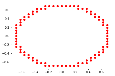
  is a computable function. For example, take the unit circle in
  .
. ![\[\mathbb{S}^1 = \{(x,y): x^2 + y^2 =1\}\]](https://konrad.burnik.org/wordpress/wp-content/ql-cache/quicklatex.com-d080c9c7c0df9960c0870bc49a444e40_l3.png "Rendered by QuickLaTeX.com")
![\[d((x,y), \mathbb{S}^1) = |x^2 + y^2 - 1|, \forall x,y \in \mathbb{R}^2.\]](https://konrad.burnik.org/wordpress/wp-content/ql-cache/quicklatex.com-5700fe7f0ac21cebea58fa05eb6e6a04_l3.png "Rendered by QuickLaTeX.com")