Investigations into infinite metric bases (Part 1/2)

Let $(X,d)$ be a metric space. Let $A \subseteq X$ be such that for all $x,y \in X$ the following implication holds:

$\left(\forall a \in A \ d(x,a) = d(a,y) \right) \implies x=y$

then we say $A$ is a metric base for $(X,d)$ . A sequence $\alpha$ in $X$ is called a dense sequence iff $\mathrm{Im}\ \alpha$ is a dense set. A metric base $A$ is a finite metric base iff $A$ is a finite set. Finding a finite metric base (if it exists) in a general metric space is already an interesting challenge and this will be explored in more detail in another post. Some information about how finite metric bases relate to computability can be found in another post. The question of existence of infinite metric bases however seems a bit less challenging due to the following easy result.

Proposition: Let $(X,d)$ be a metric space. Let $\alpha$ be a dense sequence in $X$ . Then $\mathrm{Im}\ \alpha$ is a metric base for $(X,d)$ .

Proof. Let $\alpha$ be a dense sequence and set $A = \mathrm{Im}\ \alpha$ . Let $x,y\in X$ . Suppose $d(x,a) = d(y,a)$ for all $a \in A$ . Since $\alpha$ is dense, there exists a sequence $(\beta_i)$ in $A$ such that $\lim_i \beta_i = x$ . This is equivalent to $\lim_i d(\beta_i, x) =0$ . Since $d(x,a) = d(y,a)$ for all $a \in A$ we have $\lim_i d(\beta_i, y) = 0$ .

Set $x_i=0$ , $y_i =d(x,y)$ and $z_i = d(x,\beta_i) + d(\beta_i, y)$ for all $i \in \mathbb{N}$ . From the triangle inequality and non-negativity of the metric we now have $x_i \leq y_i \leq z_i$ for all $i \in \mathbb{N}$ .

Since $\lim_i x_i = 0$ and $\lim_i z_i = 0$ , we have by the squeeze theorem $\lim_i y_i = \lim_i d(x,y) = 0$ , therefore $d(x,y) =0$ which implies $x=y$ . We conclude that $A$ is a metric base for $(X,d)$ .

Q.E.D.

Obviously, by set inclusion we have that every $A\subseteq X$ that contains a metric base is a metric base. What about metric bases which are not dense in $X$ and also do not contain a finite metric base? Formally, we have the following question:

Question: Does there exist a metric space $(X,d)$ such that it has an infinite metric base $A$ with the following properties:

$A$ is not dense;
for all finite metric bases $B$ of $(X,d)$ we have $B \not \subseteq A$ ?

Centrosymmetric QR decomposition and its connection to split-complex matrices

Introduction

Back in 2015 I published an article [1] about the QR decomposition of a centrosymmetric real matrix. In 2016 I started thinking about the meaning of this decomposition and centrosymmetric matrices in general. I discovered that centrosymmetric matrices have a natural interpretation as split-complex matrices and even more, that the centrosymmetric QR decomposition of a matrix actually corresponds to a QR decompositon of a split-complex matrix for which the original matrix is it representation. In a certain sense, the centrosymmetric QR decomposition introduced in [1] of a real square matrix of order $2n$ is equivalent to a QR decomposition of a corresponding split-complex square matrix of order $n$ . All these notions will be made precise in the following sections. This blog post is based on my own preprint.

Matrix representations

If $V$ is a finite-dimensional vector space then we denote by $\mathcal{L}(V)$ the set of all linear transformations $V \rightarrow V$ . Recall that if $V$ is an $n$ -dimensional vector space and $\mathcal{B} = (v_1,\dots,v_n)$ an ordered basis for $V$ , then every linear transformation $T : V \rightarrow V$ has an $n \times n$ matrix representation with respect to $\mathcal{B}$ denoted $[T]_\mathcal{B}$ . Further, for any two linear transformations $S, T: V \rightarrow V$ we have $[S \circ T]_\mathcal{B} = [S]_\mathcal{B} [T]_\mathcal{B}$ . The standard ordered basis for $\mathbb{R}^n$ i.e. the basis $(e_1,\dots,e_n)$ is defined as $e_{i,j} = 1$ if $i=j$ and $e_{i,j} =0$ otherwise.

An algebra $\mathfrak{A}$ is an ordered pair $(A, \cdot)$ such that $A$ is a vector space over a field $K$ and $\cdot: A \times A \rightarrow A$ is a bilinear mapping called multiplication.

Let $\mathfrak{A} = (A, \cdot)$ be an algebra. A representation of $\mathfrak{A}$ over a vector space $V$ is a map $\phi : A \rightarrow \mathcal{L}(V)$ such that

$\phi(a_1 \cdot a_2) = \phi(a_1) \circ \phi(a_2)$ for all $a_1, a_2 \in A$ .

Let $M_n(\mathbb{R})$ denote the set of $n \times n$ real matrices. If $V$ is an $n$ -dimensional vector space and $\mathcal{B} = (v_1,\dots,v_n)$ an ordered basis for $V$ then every linear transformation $T : V\rightarrow V$ has a matrix representation $[T]_\mathcal{B} \in M_n(\mathbb{R})$ . For each $a \in A$ we have $\phi(a) \in \mathcal{L}(V)$ . Since $V$ is $n$ -dimensional, we have and ordered basis $\mathcal{B}$ and $[\phi(a)]_\mathcal{B} \in M_n(\mathbb{R})$ . A matrix representation of $\mathfrak{A}$ with respect to $\mathcal{B}$ } is a map $\phi_\mathcal{B} : A \rightarrow M_n(\mathbb{R})$ such that $\phi_\mathcal{B}(a) = [\phi(a)]_\mathcal{B}$ for all $a \in A$ . Further, we have $\phi_\mathcal{B}(a_1 \cdot a_2) = \phi(a_1)_\mathcal{B}\cdot \phi(a_2)_\mathcal{B}$ for all $a_1,a_2 \in A$ . These are all well known notions from representation theory, for further information, one can consult one of the standard textbooks, for example see [3].

Algebra of split-complex numbers

Let $\Cs = (\mathbb{R}^2, \cdot)$ , where $\cdot : \mathbb{R}^2 \times \mathbb{R}^2 \rightarrow \mathbb{R}^2$ is given by

(1) $\begin{align*}(a, b) \cdot (c, d) &= (ac + bd, ad + bc)\end{align*}$

for all $(a, b), (c, d) \in \mathbb{R}^2$ . It is straightforward to verify that $\mathfrak{D}$ is
an algebra. This is the well known algebra of split-complex numbers. The split-complex numbers are also sometimes known as hyperbolic numbers.
Similarly as for the complex numbers, each real number $x \in \mathbb{R}$ can be identified with the pair $(x, 0)$ .
With this correspondence, the pair $j \equiv (0, 1)$ has the property $j^2 = +1$ and $j \not = \pm 1$ . Due to this property, $j$ is called the hyperbolic unit.
Since $(x, y) = (x, 0) + (0, 1) \cdot (0, y)$ , in the following we shall denote a pair $(x, y)$ simply with $x + j y$ . The conjugate of $z = a + j b$ is defined as $z^* = a - j b$ .

For a hyperbolic number $z = a + j b$ we define the real part as $\Real(z) = a$ and hyperbolic part as $\Hyp(z) = b$ .
For the module we set $|z| = zz^* = a^2 - b^2$ and we have $|w \cdot z| = |w|\cdot|z|$ for all $w, z \in \Cs$ .
For an extensive overview of the theory of hyperbolic numbers as well of their usefulness in Physics one can check the literature, for example [2]. For the rest of this blog post, we shall refer to these numbers as split-complex numbers.

Centrosymmetric representation of split-complex matrices

By $\M{n}$ we denote the set of all $n \times n$ split-complex matrices i.e. matrices in which entries are split-complex numbers. Note that $Z \in \M{n}$ if and only if there exist $n \times n$ real matrices $A$ , $B$ such that $Z = A + jB$ . If $A$ is a matrix then its transpose is defined as $a_{i,j}^T = a_{j,i}$ for all $i,j$ and is denoted with $A^T$ . In the following we denote by $I_n$ the $n \times n$ identity matrix and by $O_n$ the $n \times n$ zero matrix. Let $J \in M_n(\mathbb{R})$ be defined as $J = \mathrm{antidiag}(1,\dots,1)$ for each $n$ . Note that $J^2 = I$ . A matrix $R \in M_n(\mathbb{R})$ is upper-triangular if $r_{i,j} = 0$ for all $i > j$ .
A real matrix $R$ is centrosymmetric if $RJ = JR$ . An overview of centrosymmetric matrices can be found in [4]. We denote by $\CsMat{n}$ the set of all $n \times n$ centrosymmetric real matrices.

For the algebra $\Cs$ of split-complex numbers the well-known matrix representation ${cs} : \Cs \rightarrow M_{2}(\mathbb{R})$ with respect to $(e_1, e_2)$ is given by

(2) $\begin{equation*}{cs}(z) = \begin{bmatrix} \Real(z) & \Hyp(z) \\ \Hyp(z) & \Real(z) \end{bmatrix},\qquad \forall z \in \Cs.\end{equation*}$

It is straightforward to check that for all $w, z \in \Cs$ we have $\CsEmb{w \cdot z} = \CsEmb{w} \CsEmb{z}$ .

Further, on the vector space $M_n(\Cs)$ there is a natural multiplication operation $\cdot : M_n(\Cs) \times M_n(\Cs) \rightarrow M_n(\Cs)$ given by

(3) $\begin{equation*}(A + jB) \cdot (C + jD) := (AC + BD) + j(AD + BC)\end{equation*}$

for all $A,B,C,D \in M_n(\mathbb{R})$ . It is easy to verify that
$(M_n(\Cs), \cdot)$ is an algebra. In the following we refer to this algebra as the algebra of split-complex (square) matrices and denote it with $\mathfrak{M}_n$ .

Note that in the following whenever we have two matrices $A,B \in M_n(\Cs)$ , their product shall explicitly be written with a dot ' $\cdot$ ', e.g. $A \cdot B$ to indicate multiplication defined in (3). Otherwise, if $A,B \in M_n(\mathbb{R})$ we simply write $AB$ .

To state and prove our main result, we shall need the following well known characterization of centrosymmetric matrices.

Proposition 1:
Let $A \in M_{2n}(\mathbb{R})$ . Then $A \in \CsMat{2n}$ if and only if there exist $B,C \in M_{n}(\mathbb{R})$ such that

(4) $\begin{equation*}A = \begin{bmatrix}B & C J \\JC & J B J\end{bmatrix}.\end{equation*}$

Proof:
Suppose

$A =\begin{bmatrix}X & Y \\W & Z\end{bmatrix}.$

Since $A$ is centrosymmetric, we have $AJ = JA$ , or equivalently, in block-form

*** QuickLaTeX cannot compile formula:
\[\begin{bmatrix}\ & J \\J & \\end{bmatrix}\begin{bmatrix}X & Y \\W & Z\end{bmatrix} =\begin{bmatrix}X & Y \\W & Z\end{bmatrix}\begin{bmatrix}\ & J \\J & \\end{bmatrix}\]

*** Error message:
\begin{bmatrix} on input line 17 ended by \end{equation*}.
leading text: ...begin{bmatrix}\ & J \\J & \\end{bmatrix}\]
Missing $ inserted.
leading text: ...begin{bmatrix}\ & J \\J & \\end{bmatrix}\]
Missing } inserted.
leading text: ...begin{bmatrix}\ & J \\J & \\end{bmatrix}\]
Missing \cr inserted.
leading text: ...begin{bmatrix}\ & J \\J & \\end{bmatrix}\]
Missing $ inserted.
leading text: ...begin{bmatrix}\ & J \\J & \\end{bmatrix}\]
Missing } inserted.
leading text: ...begin{bmatrix}\ & J \\J & \\end{bmatrix}\]
Missing \right. inserted.
leading text: ...begin{bmatrix}\ & J \\J & \\end{bmatrix}\]
Improper \prevdepth.
leading text: \end{document}
Missing $ inserted.
leading text: \end{document}
Missing } inserted.
leading text: \end{document}

This is equivalent to

$\begin{bmatrix}JW & JZ \\JX & JY\\end{bmatrix} =\begin{bmatrix}YJ & XJ \\ZJ & WJ\end{bmatrix}$

We now have $Z = JXJ$ and $Y = JWJ$ , so

$A = \begin{bmatrix}X & JWJ \\W & JXJ\end{bmatrix}$

Now, by choosing $C = JW$ and $B = X$ and from the fact $J^2 = I$ it follows that $A$ has the form (4).

Conversely, suppose $A$ has the form (4). It can easily be shown by block-matrix multiplication that $AJ = JA$ , hence $A$ is centrosymmetric.

QED.

The map ${cs} : \M{n} \rightarrow CM_{2n}(\mathbb{R})$ defined as

(5) $\begin{equation*}{cs}(A + jB) = \begin{bmatrix}A & BJ \\JB & JAJ\end{bmatrix}\end{equation*}$

is a matrix representation of $\mathfrak{M}_n$ . We call the representation ${cs}$ the standard centrosymmetric matrix representation of $\mathfrak{M}_n$ .

Proof:
Let $W \in \M{n}$ and $Z \in \M{n}$ be such that $W = A + j B$ and $Z = C + j D$ .
We now have

$\begin{align*}\CsEmb{W} \CsEmb{Z} &= \begin{bmatrix} A & B J \\ J B & J A J \end{bmatrix} \begin{bmatrix} C & D J \\ J D & J C J \end{bmatrix} \\ &= \begin{bmatrix} A C + B D & (A D + B C) J \\ J (A D + B C) & J (A C + B D) J\end{bmatrix} = \CsEmb{W \cdot Z}\end{align*}$

which proves the claim.

QED.

Proposition.
Let $Q \in \M{n}$ . Then ${cs}(Q^T) = {cs}(Q)^T$ .

Proof.
Let $Q = A + jB$ . Then

${cs}(Q^T) = {cs}(A^T + jB^T) = \begin{bmatrix}A^T & B^T J \\J B^T & J A^T J\end{bmatrix}.$

On the other hand, keeping in mind that $J^T = J$ we have

${cs}(Q)^T = \begin{bmatrix}A & B J \\J B & JAJ\end{bmatrix}^T =\begin{bmatrix}A^T & (JB)^T \\(BJ)^T & (JAJ)^T\end{bmatrix}= \begin{bmatrix}A^T & B^T J \\J B^T & J A^T J\end{bmatrix}.$

Hence, ${cs}(Q^T) = {cs}(Q)^T$ .

QED.

Proposition.
The map ${cs}$ is a bijection.

Proof.
Injectivity. Let $Z = A + jB$ and $W = C + jD$ and $W \not = Z$ . From this,
it follows that $A \not = C$ or $B \not = D$ . Assume that $A \not = C$ . Then

$\begin{align*}\CsEmb{Z} = \begin{bmatrix}A & BJ \\JB & JAJ\end{bmatrix} & \quad &\CsEmb{W} = \begin{bmatrix}C & DJ \\JD & JCJ\end{bmatrix}.\end{align*}$

Since $A \not = C$ we have $\CsEmb{Z} \not = \CsEmb{W}$ . Let now $B \not = D$ and assume that $\CsEmb{Z} = \CsEmb{W}$ . Then from $\CsEmb{Z} = \CsEmb{W}$ it follows $JB = JD$ . Now multiplying $JB = JD$ with $J$ from the left implies $B=D$ , which is a contradiction.
We conclude that $\CsEmb{\cdot}$ is injective.

Surjectivity. Let $A \in \CsMat{2n}$ . By proposition 1 we can find matrices $B$ and $C$ such that (4) holds. But then $\CsEmb{B + jC} = A$ and since $A$ was arbitrary, we conclude that ${cs}$ is surjective.
Now, injectivity and surjectivity of ${cs}$ imply by definition that ${cs}$ is a bijection.

QED.

Correspondence of QR decompositions

Definition:
Let $A \in M_n(\Cs)$ . A pair $(Q, R)$ with $Q, R \in M_n(\Cs)$ is a QR decomposition of $A$ over $\Cs$ if the following holds:

$Q$ is orthogonal, i.e. $Q^T \cdot Q = Q \cdot Q^T = I$ ,
$R$ is upper-triangular,
$A = Q \cdot R.$

The notion of a $m\times n$ double-cone matrix was introduced by the author in [1].
Here we state the definition in block-form for the case of $H \in CM_{2n}(\mathbb{R})$ .

Definition:
Let $H \in CM_{2n}(\mathbb{R})$ . Then $H$ is a double-cone matrix iff there exist $A, B \in M_n(\mathbb{R})$ both upper-triangular such that

$H = \begin{bmatrix}A & BJ \\JB & JAJ\end{bmatrix}.$

Definition:
Let $Z \in \CsMat{n}$ . A pair $(W, Y)$ , with $W, Y \in \CsMat{n}$ is a centrosymmetric QR decomposition of $Z$ if the following holds:

$W$ is orthogonal matrix,
$Y$ is double-cone matrix,
$Z = WY.$

The algorithm to obtain an approximation of a centrosymmetric QR decomposition of a given centrosymmetric matrix $A$ was given in [1].

The following theorem provides one interpretation of the centrosymmetric QR decomposition, in the case of square centrosymmetric matrices of even order by establishing the equivalence of their centrosymmetric QR decomposition with the QR decomposition of the corresponding split-complex matrix.

Theorem 1 (QR decomposition correspondence):
Let $A \in \M{n}$ . Then $(Q,R) \in \M{n} \times \M{n}$ is a QR decomposition of $A$ if and only if

$(\CsEmb{Q}, \CsEmb{R}) \in \CsMat{2n} \times \CsMat{2n}$

is a centrosymmetric QR decomposition of $\CsEmb{A} \in \CsMat{2n}$ .

Proof.
Let $(Q, R) \in \M{n} \times \M{n}$ be a QR decomposition of $A$ .
Let $W = \CsEmb{Q}$ and $Y = \CsEmb{R}$ . We have

$\begin{align*}W = \begin{bmatrix}Q_1 & Q_2 J \\J Q_2 & J Q_1 J\end{bmatrix} & \ &Y = \begin{bmatrix}R_1 & R_2 J \\J R_2 & J R_1 J\end{bmatrix}\end{align*}$

Since $Q^T \cdot Q = I$ it follows that $\CsEmb{Q^T \cdot Q} = \CsEmb{Q^T} \CsEmb{Q} = \CsEmb{Q}^T \CsEmb{Q} = \CsEmb{I}$ .
From this we have $\CsEmb{Q}^T \CsEmb{Q} = I$ i.e. $W^T W = I$ hence $W$ is orthogonal. Since $R$ is upper-triangular and $R = R_1 + j R_2$ , then by definition we have that both $R_1$ and $R_2$ are upper-triangular. Further, $\CsEmb{R}$ is centrosymmetric by definition. From this it follows that $Y$ is centrosymmetric double-cone.
Finally, we have $\CsEmb{A} = \CsEmb{Q \cdot R} = \CsEmb{Q} \CsEmb{R}$ . Hence, $(\CsEmb{Q}, \CsEmb{R})$ is
a centrosymmetric QR decomposition of $\CsEmb{A}$ .

Conversely, let $(W, Y) = (\CsEmb{Q}, \CsEmb{R})$ . If $(W, Y)$ is a centrosymmetric QR decomposition of $\CsEmb{A}$ then $\CsEmb{A} = WY$ where $W$ is centrosymmetric and orthogonal and $Y$ is a double-cone matrix.

From the fact that $W$ is centrosymmetric we have (by Proposition 1) that

$W = \begin{bmatrix}W_1 & W_2 J \\J W_2 & J W_1 J\end{bmatrix}$

Now the property of $W$ being orthogonal i.e. the condition $W^T W = I$ implies

(6) $\begin{equation*}\begin{bmatrix}W_1^T W_1 + W_2^T W_2 & (W_1^T W_2 + W_2^T W_1) J \\J(W_2^T W_1 + W_1^T W_2) & J(W_2^T W_2 + W_1^T W_1) J\end{bmatrix}= \begin{bmatrix}I & \ \\\ & I\end{bmatrix}.\end{equation*}$

On the other hand, we have

(7) $\begin{align*}Q = W_1 + j W_2 & \ & R = Y_1 + j Y_2\end{align*}$

First we prove that $Q$ is orthogonal. From (6) we obtain

$\begin{align*}Q^T \cdot Q &= (W_1 + j W_2)^T \cdot (W_1 + j W_2) \\&= (W_1^T + j W_2^T) \cdot (W_1 + j W_2) \\& = W_1^T W_1 + W_2^T W_2 + j (W_1^T W_2 + W_2^T W_1) \\& = I + jO = I.\end{align*}$

The matrix $Y$ is centrosymmetric and double-cone which implies

$Y = \begin{bmatrix}Y_1 & Y_2 J \\J Y_2 & J Y_1 J\end{bmatrix}$

where both $Y_1$ and $Y_2$ are upper-triangular. This now implies that ${cs}^{-1}(Y) = Y_1 + j Y_2$ is upper-triangular.

Finally, let us prove that $QR = A$ . We have

$Q \cdot R = {cs}^{-1} (W) {cs}^{-1} (Y) = {cs}^{-1}(WY) = {cs}^{-1}(\CsEmb{A}) = A.$

We conclude that $(Q, R)$ is a QR decomposition of $A$ .
QED.

Example:
Let

$A = \begin{bmatrix}1 + 2j & 2 + 3j \\3 + 4j & 4 + 5j\end{bmatrix}.$

Note that $A = W + jZ$ where

(8) $\begin{align*}W = \begin{bmatrix}1 & 2 \\3 & 4\end{bmatrix} & \mbox{ and } Z = \begin{bmatrix}2 & 3 \\4 & 5\end{bmatrix}.\end{align*}$

We have

${cs}(A) = {cs}(W + jZ) = \begin{bmatrix}W & ZJ \\JZ & JWJ\end{bmatrix}= \begin{bmatrix}1 & 2 & 3 & 2 \\3 & 4 & 5 & 4 \\4 & 5 & 4 & 3 \\2 & 3 & 2 & 1\end{bmatrix}$

By applying the $\textsc{CentrosymmetricQR}$ algorithm from [1] to ${cs}(A)$ we obtain the approximations:

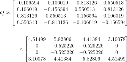
$\begin{align*}Q \approx \begin{bmatrix}-0.156594 & -0.106019 & -0.813126 & 0.550513 \\0.106019 & -0.156594 & 0.550513 & 0.813126 \\0.813126 & 0.550513 & -0.156594 & 0.106019 \\0.550513 & -0.813126 & -0.106019 & -0.156594 \\\end{bmatrix}\\\\\R \approx \begin{bmatrix}4.51499 & 5.82806 & 4.41384 & 3.10078 \\0 & -0.525226 & -0.525226 & 0 \\0 & -0.525226 & -0.525226 & 0 \\3.10078 & 4.41384 & 5.82806 & 4.51499 \\\end{bmatrix}\end{align*}$

Applying ${cs}^{-1}$ to $Q$ and $R$ yields:

$\begin{align*}{cs}^{-1}(Q) \approx \begin{bmatrix}-0.156594 & -0.106019 \\0.106019 & -0.156594\end{bmatrix} + j \begin{bmatrix}0.550513 & -0.813126 \\0.813126 & 0.550513\end{bmatrix} \\& \ & \\{cs}^{-1}(R) \approx \begin{bmatrix}4.51499 & 5.82806 \\0 & -0.525226\end{bmatrix} + j\begin{bmatrix}3.10078 & 4.41384 \\0 & -0.525226 \\\end{bmatrix}\end{align*}$

with $A \approx {cs}^{-1}(Q) \cdot {cs}^{-1}(R)$ . Now, from Theorem 1 we conclude that $({cs}^{-1}(Q), {cs}^{-1}(R))$ is an approximation of a QR decomposition of $A$ .

Conclusion

We introduced the standard centrosymmetric representation ${cs}$ for split-complex matrices. Using this representation we proved that a QR decomposition of a square split-complex matrix $A$ can be obtained by calculating the centrosymmetric QR decomposition introduced by the author in [1] of its centrosymmetric matrix representation ${cs}(A)$ .

References

Burnik, Konrad. A structure-preserving QR factorization for centrosymmetric real matrices,
Linear Algebra and its Applications 484(2015) 356 - 378
Catoni, Francesco and Boccaletti, Dino and Cannata, Roberto and Catoni, Vincenzo and Zampeti, Paolo, Hyperbolic Numbers. Geometry of Minkowski Space-Time Springer Berlin Heidelberg Berlin, Heidelberg, (2011) 3–23 ISBN: 978-3-642-17977-8
Curtis, Charles W.; Reiner, Irving. Representation Theory of Finite Groups and Associative Algebras, John Wiley & Sons (Reedition2006 by AMS Bookstore), (1962) ISBN 978-0-470-18975
James R. Weaver. Centrosymmetric (Cross-Symmetric) Matrices,Their Basic Properties, Eigenvalues, and Eigenvectors, The American Mathematical Monthly, Mathematical Association of America, (1985) 10-92, 711–717 ISSN: 00029890, 19300972 doi:10.2307/2323222

QR_decomposition_of_split_complex_matric

Two questions related to computability structures on the unit square

The following questions were proposed to me by professor Zvonko Iljazović.

Let $I = [0,1]$ . We define the metric $d_\infty$ be the metric defined as

$d_\infty((x_1,x_2), (y_1,y_2)) = \max (|x_1 - y_1|, |x_2 - y_2|).$

for all $(x_1,x_2), (y_1,y_2) \in I^2$ . Let $\mathcal{M} = (I^2, d_\infty)$ .

Let $a = (0,0)$ and $b = (0,1)$ . Suppose $(x_i)$ is a sequence in $\mathcal{M}$ such that the sequences $d(x_i, a)$ and $d(x_i,b)$ are computable sequences $\mathbb{N} \rightarrow \mathbb{R}$ ? Does the sequence $(x_i)$ need to be computable in the sense that its components are computable sequences $\mathbb{N} \rightarrow \mathbb{R}$ ?

Rendered by QuickLaTeX.com

Let $w = (1, \gamma)$ where $0 < \gamma < 1$ is an incomputable real. Then $d_\infty(x_i, a) = d_\infty(x_i, b)=1$ however, $(x_i)$ is not a computable sequence.

Now the second question. Let $a=(0,0)$ , $b=(0,1)$ and $c=(1,0)$ . Let $(x_i)$ be a sequence such that $d_\infty(x_i,a)$ , $d_\infty(x_i,b)$ and $d_\infty(x_i,c)$ are computable sequences $\mathbb{N} \rightarrow \mathbb{R}$ . Does the sequence $(x_i)$ need to be computable?

The answer is yes. The proof is available in our upcoming publication "Dense Computability Structures".

Proposition:
The metric space $\mathcal{M}$ has at least two maximal computability structures in which points $a=(0,0)$ and $b=(0,1)$ are computable.

Proof:
Let $(q_j)$ be a computable sequence in $\mathbb{R}^2$ such that $\mathrm{Im}\ q = \mathbb{Q}^2 \cap \mathcal{M}$ . Let $S_q$ be a computability structure induced by $q$ . Since $S_q$ is separable, it is also maximal.

Let $c = (1,\gamma)$ where $\gamma \in \langle 0,1 \rangle$ is an incomputable real. Then the finite sequence $(a,b,c)$ has the property $d_\infty(a,b) = d_\infty(a,c) = d_\infty(b,c) = 1$ hence by definition $(a,b,c)$ is an effective finite sequence.
Therefore,

$T = \{(a,a,a,\dots), (b,b,b,\dots), (c,c,c,\dots)\}$

is a computability structure and there exists a maximal computability structure $M$ such that $T \subseteq M$ and $a,b,c$ are computable points in $M$ .

On the other hand, the point $c$ is not computable in $S_q$ since that would contradict the fact that $w$ is a non-computable real. This is equivalent to the fact that $(c,c,c,\dots) \not \in S_q$ . Therefore, $M \not = S_q$ . From this we conclude that $M$ and $S_q$ are two maximal computability structures on $\mathcal{M}$ in which points $a$ and $b$ are computable.

Finite metric bases and computability structures

Leave a reply

Introduction

In July 2018 professor Zvonko Iljazović and myself have attended the CCA 2018 conference and presented our joint work titled "Effective compactness and uniqueness of maximal computability structures". The original presentation can be found here.

Computability structures

In the following I will mention the elements of the theory of computability structures needed to state our main result. These notions are already well known, the main contributing articles for this theory that were used for our work are listed in the references.

Let $(X,d)$ be a metric space and $(x_i)$ a sequence in $X$ . We say $(x_i)$ is an effective sequence in $(X, d)$ if the function $\mathbb{N}^2 \rightarrow \mathbb{R}$

$(i,j) \mapsto d(x_i, x_j)$

is recursive.

A finite sequence $x_0,\dots,x_n$ is an effective finite sequence if $d(x_i, x_j)$ is a recursive real number for each $i,j \in \{0, \dots, n\}$ .

If $(x_i)$ and $(y_j)$ are sequences in $X$ , we say $((x_i), (y_j))$ is an effective pair in $(X,d)$ and write $(x_i) \diamond (y_j)$ if the function $\mathbb{N}^2 \rightarrow \mathbb{R}$ ,

$(i,j) \mapsto d(x_i, y_j)$

is recursive.

Let $(X,d)$ be a metric space and $(x_i)$ a sequence in $X$ . A sequence $(y_i)$ is computable w.r.t $(x_i)$ in $(X,d)$ iff there exists a computable $F:\mathbb{N}^2\rightarrow \mathbb{N}$ such that

$d(y_i, x_{F(i, k)}) < 2^{-k}$

for all $i,k \in \mathbb{N}$ . We write $(x_i) \preceq (y_j)$ .

Let $(X, d)$ be a metric space. A set $\mathcal{S} \subseteq X^\mathbb{N}$ is a computability structure on $(X,d)$ if the following holds:

$(x_i), (y_j) \in \mathcal{S}$ , then $(x_i) \diamond (y_j)$
if $(x_i) \in \mathcal{S}$ and $(y_j) \preceq (x_i)$ , then $(y_j) \in \mathcal{S}$

We say $x$ is a computable point in $\mathcal{S}$ iff $(x,x,\dots) \in \mathcal{S}$ .

A computability structure $\mathcal{S}$ such that there exists a dense sequence $\alpha \in \mathcal{S}$ is called separable.

We say $\mathcal{S}$ is a maximal computability structure on $(X, d)$ if there exists no computability structure $\mathcal{T}$ such that $\mathcal{S} \subseteq \mathcal{T}$ and $\mathcal{S} \not = \mathcal{T}$ .

The main question

The main question we are asking and trying to answer is the following:

Question:Let $(X,d)$ be a metric space. Let $a_0,\dots,a_k \in X$ . Let $\mathcal{M}$ be a maximal computability structure in which $a_0,\dots,a_k$ are computable. Under which conditions is such $\mathcal{M}$ unique?

A known result for sub-spaces of the Euclidean space

Let $V$ be a real vector space. Let $a_0,\dots,a_k$ be vectors in $V$ . We say that $a_0,\dots, a_k$ are geometrically independent points if $a_1 - a_0, \dots, a_k - a_0$ are linearly independent vectors.

Let $X \subseteq V$ . The largest $k \in \mathbb{N}$ such that that there exist geometrically independent points $a_0,\dots, a_k \in X$ we call the affine dimension of $X$ , and write $\mathrm{dim}\ X = k$ .

The following result from [1] already answers the main question in the case where $(X,d)$ is a sub-space of the Euclidean space.

Theorem: Let $X \subseteq \mathbb{R}^n$ , $k = \mathrm{dim}\ X$ and $k \geq 1$ . If $a_0,\dots,a_{k-1}$ is a geometrically independent effective finite sequence on $X$ then there exists an unique maximal computability structure on $X$ in which $a_0,\dots,a_{k-1}$ are computable points.

Main result for more general metric spaces

We wanted to introduce for general metric spaces a notion which will be a sort of replacement to the notion of geometric independence.

In the original presentation we used the term nice sequence. It turns out that this notion is a special case of the well-known notion of a metric base.

Let $(X, d)$ be a metric space. A subset $S \subseteq X$ is called a metric base for $(X,d)$ iff for all $x,y \in X$ the following implication holds: $d(x,s) = d(y,s)$ for all $s \in S$ implies $x=y$ .

A metric space $(X,d)$ is said to be effectively compact if there exist an effective separating sequence $\alpha$ in $(X,d)$ and a computable function $f:\mathbb{N}\rightarrow \mathbb{N}$ such that

$X=B(\alpha _{0} ,2^{-k})\cup \dots \cup B(\alpha _{f(k)},2^{-k})$

for each $k\in \mathbb{N}$ . It is known that if $(X,d)$ is effectively compact, then for each effective separating sequence $\alpha$ in $(X,d)$ there exists such a computable function $f$ .

A metric base is exactly the notion we needed to obtain the following result, at least for effectively compact metric spaces.

Theorem: Let $(X,d)$ be an effectively compact metric space. Suppose $a_{0} ,\dots ,a_{n}$ is a metric base in $(X,d)$ and suppose that there exists a separable computability structure $\mathcal{S}$ on $(X,d)$ in which $a_{0} ,\dots ,a_{n}$ are computable points. Then $\mathcal{S}$ is a unique maximal computability structure on $(X,d)$ in which $a_{0} ,\dots ,a_{n}$ are computable points.

In fact, an even more general form of the theorem holds: the assumption of effective compactness of the space $(X,d)$ can be replaced with the assumption that $(X,d)$ has compact closed balls and there exists $\alpha$ such that the computable metric space $(X,d,\alpha)$ has the effective covering property.

Proofs will be presented in our future up-coming publication.

References

Zvonko Iljazović. Isometries and Computability Structures. Journal of Universal Computer Science, 16(18):2569--2596, 2010.
Zvonko Iljazović and Lucija Validžić. Maximal computability structures. Bulletin of Symbolic Logic, 22(4):445--468, 2016.
Alexander Melnikov. Computably isometric spaces. Journal of Symbolic Logic, 78:1055--1085, 2013.
Marian Pour-El and Ian Richards. Computability in Analysis and Physics. Springer-Verlag, Berlin-Heielberg-New York, 1989.
Klaus Weihrauch. Computable Analysis. Springer, Berlin, 2000.
M. Yasugi, T. Mori and Y. Tsujji. Effective properties of sets and functions in metric spaces with computability structure. Theoretical Computer Science}, 219:467--486, 1999.
M. Yasugi, T. Mori and Y. Tsujji. Computability structures on metric spaces. Combinatorics, Complexity and Logic Proc. DMTCS96 (D.S.~Bridges et al), Springer, Berlin}, 351--362, 1996.

Hyperbolic numbers and fractals

What happens when we change the identity defining the imaginary unit for the complex numbers $i^2=-1$ to $i^2=1$ and enforcing i different from 1? We get the somewhat less known numbers called hyperbolic or split-complex numbers. The most common thing about complex numbers that comes to mind are the nice pictures of fractals and there are plenty of tools already out there to generate them. However, for the hyperbolic numbers there aren't as much fractal generators out there, so let us now make a simple tool in Python to generate these fractals as well.

First, we need to implement the basic arithmetic with hyperbolic numbers. This will enable us to write simple arithmetic expressions like z**2 + c directly instead of writing out the expressions in component form using real and imaginary parts. I made a simple Python implementation of class HyperbolicNumber in module hyperbolic doing exactly this. Using this module, we can now write a function for counting the number of iterations of f(z)=z**2+c before "escaping to infinity" in a straightforward way. In fact the formula is identical to the escape-time algorithm for fractals over complex numbers.

from hyperbolic import HyperbolicNumber

def f(z):
    w = z
    total = 0
    while mag(w) < 2.0 and total < 300:
        w = w**2 + z
        total += 1
    return total

Basically, the above function is all we need to start generating images of fractals. Here of course, we focus only on the famous map family { f_c(z) = z**2+c} indexed by c, but any other could be used as well. We add an additional parameter to f(z) to become f(z,c) and encapsulate it in the HyperbolicFractal class. This class will be our abstraction for a fractal calculation, which basically just calculates a 2**-k approximation of the Julia set of f_c over some given rectangular region in the hyperbolic number plane. For all the points z of a given rectangular range [centerx-rangex, centerx+rangex]x[centery-rangey, centery+rangey] we perform the call to f(z, c). To avoid recalculation every time of the same region, or part of a region, points which have already been calculated are stored in an internal cache so any subsequent calls to f(z, c) are just looked up instead of being recalculated. Here's the code.

import numpy
import matplotlib.cm as cm
import matplotlib.pylab as plt
from hyperbolic import HyperbolicNumber

class HyperbolicFractal:
    def __init__(self):
        self.hits = 0
        self.cache = {}
        
    def f(self, z, c):
        if (z, c) in self.cache:
            self.hits += 1
            return self.cache[(z, c)]
        w = z
        total = 0
        while mag(w) < 2.0 and total < 300:
            w = w**2 + c
            total += 1
        self.cache[(z, c)] = total
        return self.cache[(z, c)]

    def show(self, scale, centerx, centery, rangex, rangey, c):
        """Draw a 2**(-scale) approximation of a hyperbolic fractal 
        over a given rectangular range."""
        self.hits = 0
        totals = (centerx+rangex - (centerx-rangex))\
        * (centery+rangey - (centery-rangey))
        t = [[self.f((1.0/(2**scale)) * HyperbolicNumber(x,y), c)\
        for x in range(centerx-rangex, centerx+rangex)]\
        for y in range(centery-rangey, centery+rangey)]
        matrix = numpy.matrix(t)
        fig = plt.figure()
        plt.imshow(matrix, interpolation='bilinear', cmap=cm.RdYlGn, origin='center')
        print ("Total: {} Cache hits: {} Cache hit ratio: {}".format(totals, self.hits, (1.0 * self.hits)/totals))
        plt.show()

Let's try it out.

H = HyperbolicFractal()
H.show(7, 0, 0, 200, 200, HyperbolicNumber(-20/2**3, 0))

And there you have it! We now have a tool to look into the hyperbolic number world.

The full code for this implementation can be found on Github.

Computable Sets in the Euclidean plane using Python

#####################################################################
#
# Implementing the notion of Computable Set in the euclidean plane 
#
# Every weakly computable set in the euclidean plane is a set 
# of zeroes of some a computable function.
#
# Konrad Burnik, June 2017.
#
#####################################################################

from math import *
from decimal import *
import matplotlib.pyplot as plt

class ComputableSet:
    '''A computable subset of the euclidean plane is given by its computable function representing it.'''
    def f(self, x, y):
        '''A function whose zeroes represent this computable set. 
           For example: def f(x, y): return x**2 + y**2 - 1 has zeroes which represents a unit circle.
        '''
        raise Exception("Not implemented!")
    
    def points(self, k):
        return [(x/2**k, y/2**k) 
                        for y in range(-2**k, 2**k + 1) 
                        for x in range(-2**k, 2**k + 1) 
                        if Decimal(-1) / Decimal(2**k) < self.f(Decimal(x)/Decimal(2**k), Decimal(y)/Decimal(2**k)) < Decimal(1) / Decimal(2**k)]  class Circle(ComputableSet):
    def f(self, x, y):
        return x**2 + y**2 - Decimal(1/2)
class EllipticCurve(ComputableSet):
    def f(self, x, y):
        return x**2 + y**3 - Decimal(1/2)

def plot_set(s, k):
    points = s.points(k)
    x = list(map(lambda x : x[0], points))
    y = list(map(lambda x : x[1], points))

    plt.plot(x, y, 'ro')
    plt.show()

class Circle(ComputableSet):
    def f(self, x, y):
        return x**2 + y**2 - Decimal(1/2)

class EllipticCurve(ComputableSet):
    def f(self, x, y):
        return x**2 + y**3 - Decimal(1/2)

class ComputableSetUnion(ComputableSet):
    def __init__(self):
        self.A = ComputableSet()
        self.B = ComputableSet()
        
    def f(self, x, y):
        return self.A.f(x, y) * self.B.f(x, y)

Computable metric spaces in a nutshell

Leave a reply

What are computable metric spaces?

We can generalize the notions of computability over the reals and in the euclidean space to metric spaces. A computable metric space is a triple $(X,d,\alpha)$ where $(X,d)$ is a metric space and $\alpha$ is a sequence in $X$ such that its image is dense in $X$ and the function $\mathbb{N}^2 \rightarrow \mathbb{R}$ defined as $(i,j) \mapsto d(\alpha_i, \alpha_j),\ \forall i,j\in\mathbb{N}$ is computable. For example, a definition of computable point is a generalization of the computable real: A point $x \in X$ is computable in $(X,d,\alpha)$ if there exists a computable function $f:\mathbb{N} \rightarrow \mathbb{N}$ such that $d(\alpha_{f(k)}, x) < 2^{-k}$ for every $k \in \mathbb{N}$ . Similarly, we can define a computable sequence of points in $X$ and functions between metric spaces that are computable,... but for subsets of $X$ it is not the same as definition of computability in $\mathbb{R}^n$ but it borrows the definitions from classical recursion theory. First we fix some computable enumeration of rational balls in $X$ for example let $(I_i)$ be a fixed such enumeration. Then for a set $S \subseteq X$ we say that $S$ is recursively enumerable $T = \{i \in \mathbb{N} | S \cap I_i \not = \emptyset\}$ is recursively enumerable i.e. there exists a computable function $f:\mathbb{N} \rightarrow \mathbb{N}$ such that $f(\mathbb{N}) = T$ . A subset $S$ is co-recursively enumerable if we have an algorithm that covers the complement of $S$ with rational balls. In other words, $S$ is co-recursively computable iff there exists a recursively enumerable subset $A$ of $\mathbb{N}$ such that $X \setminus S = \bigcup_{i \in A} I_i$ . A subset $S$ is computable iff $S$ is recursively computable and co-recursively computable.

We can of course generalize further and define computable topological spaces but I shall not go further into that. That is a topic for another post. Note that as we generalize more and more there are pathological spaces that do not have nice computability properties and must be more and more careful when dealing with computability.

Introduction to computable analysis (Part 1/2)

Leave a reply

What is Computable analysis anyway?

Roger Penrose in his book "The emperors new Mind" asked an interesting question regarding the Mandelbrot set: "Is the Mandelbrot set recursive?" The term "recursive" is an old name for "computable" and has nothing to do with recursion in programming.

The Mandelbrot Set (zoomed in)

Classical computability theory (also known as recursion theory) is a branch of mathematical logic that deals with studying what functions $\mathbb{N}\rightarrow \mathbb{N}$ are computable. Computable analysis is in some sense an extension of this theory. It is a branch of mathematics that applies computability theory to problems in mathematical analysis. It is concerned with questions of effectivity in analysis and its main goal is to find what parts of analysis can be described by an algorithmic procedure, one of the basic questions being what functions $f:\mathbb{R}\rightarrow\mathbb{R}$ are computable? (note the domain and codomain are now the reals).

Computable reals

Suppose we take a real number $x$ . Is $x$ computable? What do we mean by $x$ being computable? If we can find an algorithm $A$ that calculates for each input $k \in \mathbb{N}$ a rational approximation $A_k$ of $x$ ; and such that the sequence $(A_k)$ "converges fast" to $x$ then we say that $x$ is a computable real. More precisely, a real number $x \in R$ is computable iff there exists a computable function $f:\mathbb{N} \rightarrow \mathbb{Q}$ such that $|f(k) - x| < 2^{-k}$ for each $k \in \mathbb{N}$ . For example, every rational number is computable. The famous number $\pi$ is computable, and in our previous post we proved that $\sqrt{2}$ is computable. It turns out that the set of computable reals, denoted by $\mathbb{R}_C$ is a field with respect to addition and multiplication. But there exist real numbers which are not computable. This is easy to see as there is only a countable number of computable functions $\mathbb{N}\rightarrow\mathbb{N}$ , and since we know that $\mathbb{R}$ is uncountable, so we have more real numbers than we have possible algorithms, we conclude that there must be a real number that is not computable. One example of an uncomputable real is the limit of a Specker sequence. And one other interesting one is the Chaitin constant. In fact, if we take any recursively enumerable but non-recursive set $A \subseteq \mathbb{N}$ , then the number $\alpha = \sum_{i \in A} 2^{-i}$ is an example of a real number which is not computable.

Computable sequences of reals

If we have a sequence of computable reals $(x_n)$ (and hence a sequence of algorithms) we may ask if this sequence is computable i.e. is there a single algorithm that describes the whole sequence? If there exists a computable function $f : \mathbb{N}^2 \rightarrow \mathbb{Q}$ such that

$|f(n,k) - x_n| < 2^{-k}$

for each $n,k \in \mathbb{N}$ then we say that $(x_n)$ is a computable sequence. We have seen that each rational number is computable, but this is not true for sequences of rational numbers! One example of a sequence that has each term computable but it is not uniformly computable is the following:

Computable real functions

Real functions which are a main object of study in analysis can be studied in this computability setting, a function $f:\mathbb{R} \rightarrow \mathbb{R}$ is computable iff

it maps computable sequences to computable sequences i.e. $f(x_i)$ is computable for every computable sequence $(x_i)$ ;
it is effectively uniformly continous i.e. if there exists a computable sequence thatdescribes the modulus of continuity of $f$ .

The fundamental theorem of computable analysis is that every computable real function is continuous.

There is also a notion of computability for the process of integration, derivation, solving partial differential equations, etc. and we shall look into that topic in another post.

Computable subsets of the Euclidean space

Unit circle approximated with dyadic points

Next, let's look at the subsets of the euclidean space $\mathbb{R}^n$ and ask a simple question: what subsets are computable? First, note that saying $S$ is computable iff its indicator function

$\chi_S(x) =\begin{cases} 1, & x \in S \\ 0, & x \not \in S \end{cases}$

is computable is not a useful definition since the indicator function is not continous except when $S =\mathbb{R}^n$ or $S=\emptyset$ . A subset $S$ of $\mathbb{R}^n$ is computable iff the function $\mathbb{R}^n \rightarrow \mathbb{R}$ defined as $x \mapsto d(x, S)$ is a computable function. For example, take the unit circle in $\mathbb{R}^2$ .

$\mathbb{S}^1 = \{(x,y): x^2 + y^2 =1\}$

. The distance function is

$d((x,y), \mathbb{S}^1) = |x^2 + y^2 - 1|, \forall x,y \in \mathbb{R}^2.$

These are just some basic definitions and facts, but also interesting questions are studied in computable analysis like for example what mappings preserve computability of objects? Is for example the Mandelbrot set computable? What about Julia Sets? For them, there are nice results presented in the book "Computability of Julia Sets" by Braverman and Yampolsky. Although Julia Sets have been thoroughly researched in the book, for the Mandelbrot set we still don't know the answer.

Basically for anything we do in analysis (finding derivatives, integration, finding roots, solving PDEs ...) we may ask: "Is it computable?" and that is a topic for another post.

(to be continued)

Another look at the square root of two

Leave a reply

The other day I was thinking about approximating $\sqrt{2}$ in terms of segments of size $1/2^k$ for $k=0,1,2,\dots$ , The question I was interested was "What is the least number of segments of length $1/2^k$ that we need to cross over $\sqrt{2}$ starting from zero?" and one particular sequence of integers I came up with was this:

$2, 3, 6, 12, 23, 46, 91, 182, 363, 725,\dots.$

Sadly, at the time of writing this post the Online Encyclopedia of Integer Sequences did not return anything for this sequence.

The sequence represents the numerators for dyadic rationals which approximate $\sqrt{2}$ within precision $2^{-k}$ (within k-bits of precision), but is this sequence computable? In what follows I assume that the reader is familiar with the basic definitions of mu-recursive functions.

It turns out that our sequence can be described by a recursive function $f: \mathbb{N} \rightarrow \mathbb{N}$

$f(k) = \mu.n [n^2 > 2^{(2k+1)}]$

for all $k\geq0$ .

The idea of the function $f$ is that for each $k$ it outputs the number of $1/2^k$ segments that fit into $\sqrt{2}$ plus one.

Since for each $k$ , the value $f(k)$ is the smallest integer such that $f(k)/2^k > \sqrt{2}$ we have

$(f(k) - 1)/2^k < \sqrt{2} < f(k)/2^k$

for each $k\geq 0$ .

From this we obtain the error bound $|f(k)/2^k - \sqrt{2}| < 2^{-k}$ .

Approximation of $\sqrt{2}$ within precision $2^{-k}$ can be "represented" by a natural number $f(k)$ . To get the actual approximation by a dyadic rational just divide by $2^k$ but what we want is to avoid division. We want to calculate only with natural numbers!

Implementation

The function f has a straightforward (although inefficient) implementation in Python.

def calcSqrt2Segments(k):
    n = 0
    while(n*n <= 2**(2*k+1)):
        n = n + 1
    return n

This is in fact terribly inefficient, but in computability theory efficiency is not the goal, the goal is usually to prove that something is uncomputable even if you have all the resources of time and space at your disposal. Nevertheless, here is a slightly better version we get if we notice that the next term $f(k+1)$ is about twice as large as $f(k)$ with a small correction.

def calcSqrt2segmentsRec(k):
    if k == 0:
        return 2
    else:
        res = 2*calcSqrt2segmentsRec(k-1) - 1
        if res*res <= 2**(2*k+1):
           res = res + 1
        return res

This of course suffers from stack overflow problems, so memoization is a natural remedy.

def calcSqrt2segmentsMemo(k):
    m = dict()
    m[0] = 2
    for j in range(1, k+1):
        m[j] = 2*m[j-1] - 1
        if m[j]*m[j] <= 2**(2*j+1):
            m[j] = m[j] + 1
    return m[k]

Memoization can use-up memory and we can do better. We don't need to memorize the whole sequence up to k to calculate $f(k+1)$ we only need the value $f(k)$ .

def calcSqrt2segmentsBest(k):
    m = 2
    for j in range(1, k+1):
        m = 2*m - 1
        if m*m <= 2**(2*j+1):
            m = m + 1
    return m

After defining a simple timing function and testing our memoization and "best" version we see that the best version is not so good in terms of running time when compared with memoization, they are both approximately about the same in terms of speed (the times are in seconds):

>>> timing(calcSqrt2segmentsMemo, 10000)
0.6640379428863525
>>> timing(calcSqrt2segmentsBest, 10000)
0.6430368423461914
>>> timing(calcSqrt2segmentsMemo, 20000)
3.3311898708343506
>>> timing(calcSqrt2segmentsBest, 20000)
3.3061890602111816
>>> timing(calcSqrt2segmentsMemo, 30000)
8.899508953094482
>>> timing(calcSqrt2segmentsBest, 30000)
8.848505973815918
>>> timing(calcSqrt2segmentsMemo, 50000)
30.04171895980835
>>> timing(calcSqrt2segmentsBest, 50000)
29.96371293067932
>>> timing(calcSqrt2segmentsMemo, 100000)
164.99343705177307
>>> timing(calcSqrt2segmentsBest, 100000)
168.6026430130005

Neverteless, we can use our "best" program to calculate $\sqrt{2}$ to arbritrary number of decimal places (in base 10). First, we need to determine how many bits are sufficient to calculate $\sqrt{2}$ to $n$ decimal places in base 10. Simple calculation yields:

$k > \lceil n log_2 10 \rceil.$

In Python we need a helper function that calculates this bound that avoids the nasty log and ceiling functions, so here it is:

def calcNumDigits(n):
    res = 1
    for j in range(2, n+1): 
        if( j%3 == 0 or j%3 == 1 ):
          res = res + 3
        else:
          res = res + 4
    return res

At last, calculating $\sqrt{2}$ to arbritrary precision is done with this simple code below, returning a String with the digits of $\sqrt{2}$ in base 10. Note once more, that all this calculation is done only with the natural numbers and here we are using Python's powerful implementation of arithmetic with arbritrary long integers (which is not as nicely supported for decimals at least at the time of writing this post).

Note also, that instead of dividing $f(k)$ by $2^k$ we are multiplying it with $5^k$ to get a natural number with all of it's digits being an approximation of $\sqrt{2}$ with k bits of precision. This natural number we are then converting to a string, inserting a decimal point '.' and returning this as our result. So, here is the code:

def calcSqrt2(n):
    k = calcNumDigits(n)
    res = str(5**k * calcSqrt2segmentsBest(k))
    return res[0:1] + '.' + res[1:n]

Running it gives us nice results:

>>> calcSqrt2(30)
'1.41421356237309504880168872421'
>>> calcSqrt2(300)
'1.41421356237309504880168872420969807856967187537694807317667973799073247846210703885038753432764157273501384623091229702492483605585073721264412149709993583141322266592750559275579995050115278206057147010955997160597027453459686201472851741864088919860955232923048430871432145083976260362799525140799'
>>> calcSqrt2(3000)
'1.41421356237309504880168872420969807856967187537694807317667973799073247846210703885038753432764157273501384623091229702492483605585073721264412149709993583141322266592750559275579995050115278206057147010955997160597027453459686201472851741864088919860955232923048430871432145083976260362799525140798968725339654633180882964062061525835239505474575028775996172983557522033753185701135437460340849884716038689997069900481503054402779031645424782306849293691862158057846311159666871301301561856898723723528850926486124949771542183342042856860601468247207714358548741556570696776537202264854470158588016207584749226572260020855844665214583988939443709265918003113882464681570826301005948587040031864803421948972782906410450726368813137398552561173220402450912277002269411275736272804957381089675040183698683684507257993647290607629969413804756548237289971803268024744206292691248590521810044598421505911202494413417285314781058036033710773091828693147101711116839165817268894197587165821521282295184884720896946338628915628827659526351405422676532396946175112916024087155101351504553812875600526314680171274026539694702403005174953188629256313851881634780015693691768818523786840522878376293892143006558695686859645951555016447245098368960368873231143894155766510408839142923381132060524336294853170499157717562285497414389991880217624309652065642118273167262575395947172559346372386322614827426222086711558395999265211762526989175409881593486400834570851814722318142040704265090565323333984364578657967965192672923998753666172159825788602633636178274959942194037777536814262177387991945513972312740668983299898953867288228563786977496625199665835257761989393228453447356947949629521688914854925389047558288345260965240965428893945386466257449275563819644103169798330618520193793849400571563337205480685405758679996701213722394758214263065851322174088323829472876173936474678374319600015921888073478576172522118674904249773669292073110963697216089337086611567345853348332952546758516447107578486024636008344491148185876555542864551233142199263113325179706084365597043528564100879185007603610091594656706768836055717400767569050961367194013249356052401859991050621081635977264313806054670102935699710424251057817495310572559349844511269227803449135066375687477602831628296055324224269575345290288387684464291732827708883180870253398523381227499908123718925407264753678503048215918018861671089728692292011975998807038185433325364602110822992792930728717807998880991767417741089830608003263118164279882311715436386966170299993416161487868601804550555398691311518601038637532500455818604480407502411951843056745336836136745973744239885532851793089603738989151731958741344288178421250219169518755934443873961893145499999061075870490902608835176362247497578588583680374579311573398020999866221869499225959132764236194105921003280261498745665996888740679561673918595728886424734635858868644968223860069833526427990562831656139139425576490620651860216472630333629750756978706066068564981600927187092921531323682'

Note:
This can of course be generalized to calculating the square root of any number and of any order. This is an easy exercise for the reader.

Computable Analysis Applied to Formal Verification of Cyber-Physical Systems

Leave a reply

The following video I found online is about combining the theory of computable analysis with formal verification methods. I find this video very interesting because my diploma/master's thesis was about formal verification while my PhD study is from the area of computable analysis, so the work presented in this video nicely combines the two areas.

Title: "Computable Real Numbers and Why They Are Still Important Today"

Author: Edmund Clarke

Description: "Talk by ACM A.M. Turing Laureate Edmund Clarke during the ACM A.M. Turing Centenary Celebration, June, 2012. Abstract: Although every undergraduate in computer science learns about Turing Machines, it is not well known that they were originally proposed as a means of characterizing computable real numbers. For a long time, formal verification paid little attention to computational applications that involve the manipulation of continuous quantities, even though such applications are ubiquitous. In recent years, however, there has been great interest in safety-critical hybrid systems involving both discrete and continuous behaviors, including autonomous automotive and aerospace applications, medical devices of various sorts, control programs for electric power plants, and so on. As a result, the formal analysis of numerical computation can no longer be ignored. This talk focuses on one of the most successful verification techniques, temporal logic model checking. Current industrial model checkers do not scale to handle realistic hybrid systems. The key to handling more complex systems is to make better use of the theory of the computable reals, and computable analysis more generally. New formal methods for hybrid systems should combine existing discrete methods in model checking with new algorithms based on computable analysis. In particular, this talk discusses a model checker currently being developed along these lines."

The Hitchhiker's Guide to Computable Mathematics

Konrad Burnik

Investigations into infinite metric bases (Part 1/2)

Centrosymmetric QR decomposition and its connection to split-complex matrices

Introduction

Matrix representations

Algebra of split-complex numbers

Centrosymmetric representation of split-complex matrices

Correspondence of QR decompositions

Conclusion

References

Two questions related to computability structures on the unit square

Finite metric bases and computability structures

Introduction

Computability structures

The main question

A known result for sub-spaces of the Euclidean space

Main result for more general metric spaces

References

Hyperbolic numbers and fractals

Computable Sets in the Euclidean plane using Python

Computable metric spaces in a nutshell

Introduction to computable analysis (Part 1/2)

Another look at the square root of two

Computable Analysis Applied to Formal Verification of Cyber-Physical Systems

Links